Getting More Information About a Clustering
Once you have the basics of clustering sorted you may want to dig a little deeper than just the cluster labels returned to you. Fortunately, the hdbscan library provides you with the facilities to do this. During processing HDBSCAN* builds a hierarchy of potential clusters, from which it extracts the flat clustering returned. It can be informative to look at that hierarchy, and potentially make use of the extra information contained therein.
Suppose we have a dataset for clustering. It is a binary file in NumPy format and it can be found at https://github.com/lmcinnes/hdbscan/blob/master/notebooks/clusterable_data.npy.
import hdbscan
import numpy as np
import matplotlib.pyplot as plt
import seaborn as sns
%matplotlib inline
data = np.load('clusterable_data.bin')
#or
data = np.load('clusterable_data.npy')
#depending on the format of the file
data.shape
(2309, 2)
data
array([[-0.12153499, -0.22876337],
   [-0.22093687, -0.25251088],
   [ 0.1259037 , -0.27314321],
   ...,
   [ 0.50243143, -0.3002958 ],
   [ 0.53822256,  0.19412199],
   [-0.08688887, -0.2092721 ]])
plt.scatter(*data.T, s=50, linewidth=0, c='b', alpha=0.25)
<matplotlib.collections.PathCollection at 0x7f6b61ad6e10>
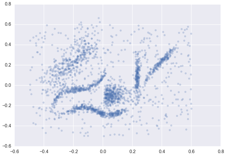
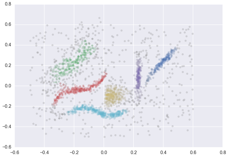
We can cluster the data as normal, and visualize the labels with different colors (and even the cluster membership strengths as levels of saturation)
clusterer = hdbscan.HDBSCAN(min_cluster_size=15).fit(data)
color_palette = sns.color_palette('deep', 8)
cluster_colors = [color_palette[x] if x >= 0
                  else (0.5, 0.5, 0.5)
                  for x in clusterer.labels_]
cluster_member_colors = [sns.desaturate(x, p) for x, p in
                         zip(cluster_colors, clusterer.probabilities_)]
plt.scatter(*data.T, s=50, linewidth=0, c=cluster_member_colors, alpha=0.25)
Condensed Trees
The question now is what does the cluster hierarchy look like – which
clusters are near each other, or could perhaps be merged, and which are
far apart. We can access the basic hierarchy via the condensed_tree_
attribute of the clusterer object.
clusterer.condensed_tree_
<hdbscan.plots.CondensedTree at 0x10ea23a20>
This merely gives us a CondensedTree object. If we want to visualize the
hierarchy we can call the plot() method:
clusterer.condensed_tree_.plot()
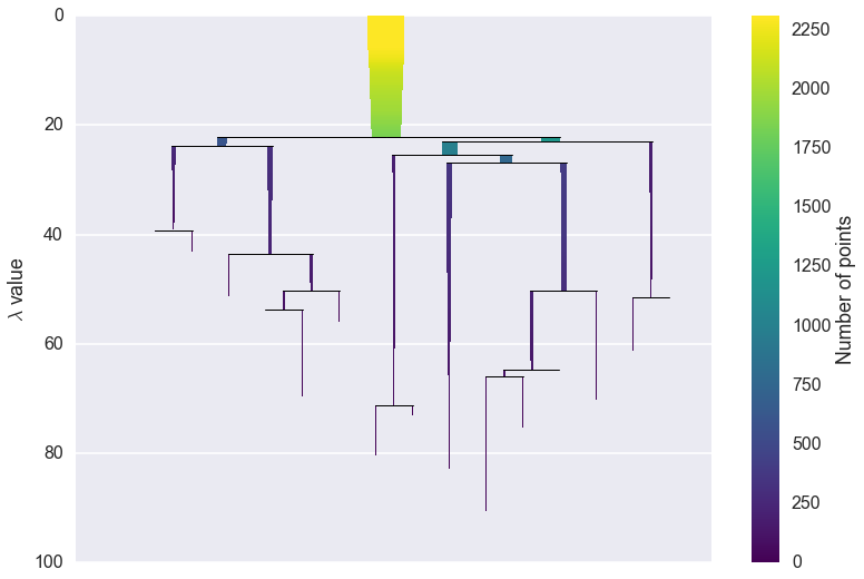
We can now see the hierarchy as a dendrogram, the width (and color) of
each branch representing the number of points in the cluster at that
level. If we wish to know which branches were selected by the HDBSCAN*
algorithm we can pass select_clusters=True. You can even pass a
selection palette to color the selections according to the cluster
labeling.
clusterer.condensed_tree_.plot(select_clusters=True,
                               selection_palette=sns.color_palette('deep', 8))
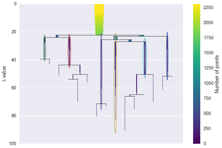
From this, we can see, for example, that the yellow cluster at the
center of the plot forms early (breaking off from the pale blue and
purple clusters) and persists for a long time. By comparison the green
cluster, which also forms early, quickly breaks apart and then
vanishes altogether (shattering into clusters all smaller than the
min_cluster_size of 15).
You can also see that the pale blue cluster breaks apart into several subclusters that in turn persist for quite some time – so there is some interesting substructure to the pale blue cluster that is not present, for example, in the dark blue cluster.
If this was a simple visual analysis of the condensed tree can tell you
a lot more about the structure of your data. This is not all we can do
with condensed trees, however. For larger and more complex datasets the
tree itself may be very complex, and it may be desirable to run more
interesting analytics over the tree itself. This can be achieved via
several converter methods: to_networkx(), to_pandas(), and
to_numpy().
First we’ll consider to_networkx()
clusterer.condensed_tree_.to_networkx()
<networkx.classes.digraph.DiGraph at 0x11d8023c8>
As you can see we get a NetworkX directed graph, which we can then use all the regular NetworkX tools and analytics on. The graph is richer than the visual plot above may lead you to believe, however:
g = clusterer.condensed_tree_.to_networkx()
g.number_of_nodes()
2338
The graph actually contains nodes for all the points falling out of
clusters as well as the clusters themselves. Each node has an associated
size attribute and each edge has a weight of the lambda value
at which that edge forms. This allows for much more interesting
analyses.
Next, we have the to_pandas() method, which returns a panda DataFrame
where each row corresponds to an edge of the NetworkX graph:
clusterer.condensed_tree_.to_pandas().head()
| parent | child | lambda_val | child_size | |
|---|---|---|---|---|
| 0 | 2309 | 2048 | 5.016526 | 1 |
| 1 | 2309 | 2006 | 5.076503 | 1 |
| 2 | 2309 | 2024 | 5.279133 | 1 |
| 3 | 2309 | 2050 | 5.347332 | 1 |
| 4 | 2309 | 1992 | 5.381930 | 1 |
Here the parent denotes the id of the parent cluster, the child
the id of the child cluster (or, if the child is a single data point
rather than a cluster, the index in the dataset of that point), the
lambda_val provides the lambda value at which the edge forms, and
the child_size provides the number of points in the child cluster.
As you can see the start of the DataFrame has singleton points falling
out of the root cluster, with each child_size equal to 1.
If you want just the clusters, rather than all the individual points
as well, simply select the rows of the DataFrame with child_size
greater than 1.
tree = clusterer.condensed_tree_.to_pandas()
cluster_tree = tree[tree.child_size > 1]
Finally we have the to_numpy() function, which returns a numpy record
array:
clusterer.condensed_tree_.to_numpy()
array([(2309, 2048, 5.016525967983049, 1),
       (2309, 2006, 5.076503128308643, 1),
       (2309, 2024, 5.279133057912248, 1), ...,
       (2318, 1105, 86.5507370650292, 1), (2318, 965, 86.5507370650292, 1),
       (2318, 954, 86.5507370650292, 1)],
      dtype=[('parent', '<i8'), ('child', '<i8'), ('lambda_val', '<f8'), ('child_size', '<i8')])
This is equivalent to the pandas DataFrame but is in pure NumPy and hence has no pandas dependencies if you do not wish to use pandas.
Single Linkage Trees
We have still more data at our disposal, however. As noted in the How
HDBSCAN Works section, prior to providing a condensed tree the algorithm
builds a complete dendrogram. We have access to this too via the
single_linkage_tree_ attribute of the clusterer.
clusterer.single_linkage_tree_
<hdbscan.plots.SingleLinkageTree at 0x121d4b128>
Again we have an object which we can then query for relevant
information. The most basic approach is the plot() method, just like
the condensed tree.
clusterer.single_linkage_tree_.plot()
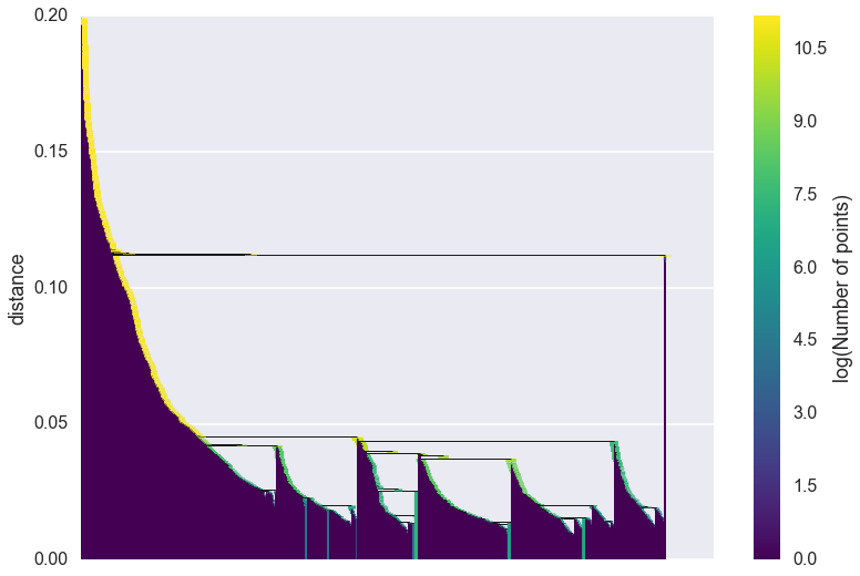
As you can see we gain a lot from condensing the tree in terms of better
presenting and summarising the data. There is a lot less to be gained
from visual inspection of a plot like this (and it only gets worse for
larger datasets). The plot function support most of the same
functionality as the dendrogram plotting from
scipy.cluster.hierarchy, so you can view various truncations of the
tree if necessary. In practice, however, you are more likely to be
interested in access the raw data for further analysis. Again we have
to_networkx(), to_pandas() and to_numpy(). This time the
to_networkx() provides a direct NetworkX version of what you see
above. The NumPy and pandas results conform to the single linkage
hierarchy format of scipy.cluster.hierarchy, and can be passed to
routines there if necessary.
If you wish to know what the clusters are at a given fixed level of the
single linkage tree you can use the get_clusters() method to extract
a vector of cluster labels. The method takes a cut value of the level
at which to cut the tree, and a minimum_cluster_size to determine
noise points (any cluster smaller than the minimum_cluster_size).
clusterer.single_linkage_tree_.get_clusters(0.023, min_cluster_size=2)
array([ 0, -1, 0, ..., -1, -1, 0])
In this way, it is possible to extract the DBSCAN clustering that would result for any given epsilon value, all from one run of hdbscan.