Predicting clusters for new points
Often it is useful to train a model once on a large amount of data, and then query the model repeatedly with small amounts of new data. This is hard for HDBSCAN* as it is a transductive method – new data points can (and should!) be able to alter the underlying clustering. That is, given new information it might make sense to create a new cluster, split an existing cluster, or merge two previously separate clusters. If the actual clusters (and hence their labels) change with each new data point it becomes impossible to compare the cluster assignments between such queries.
We can accommodate this by effectively holding a clustering fixed (after a potentially expensive training run) and then asking: if we do not change the existing clusters which cluster would HDBSCAN* assign a new data point to. In practice this amounts to determining where in the condensed tree the new data point would fall (see How HDBSCAN Works) assuming we do not change the condensed tree. This allows for a very inexpensive operation to compute a predicted cluster for the new data point.
This has been implemented in hdbscan as the
approximate_predict() function. We’ll look
at how this works below.
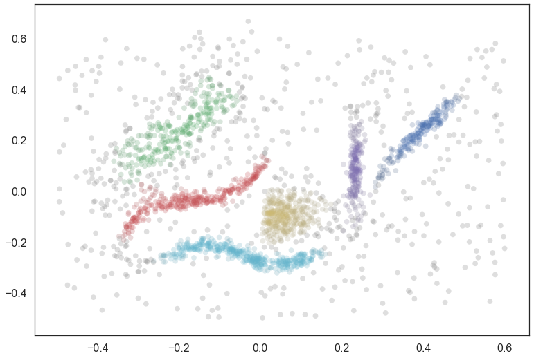
As usual we begin with our test synthetic data set, and cluster it with
HDBSCAN. The primary point to note here, however, is the use of the
prediction_data=True keyword argument. This ensures that HDBSCAN
does a little extra computation when fitting the model that can
dramatically speed up the prediction queries later.
You can also get an HDBSCAN object to create this data after the fact
via the generate_prediction_data() method.
data = np.load('clusterable_data.npy')
clusterer = hdbscan.HDBSCAN(min_cluster_size=15, prediction_data=True).fit(data)
pal = sns.color_palette('deep', 8)
colors = [sns.desaturate(pal[col], sat) for col, sat in zip(clusterer.labels_,
                                                            clusterer.probabilities_)]
plt.scatter(data.T[0], data.T[1], c=colors, **plot_kwds);
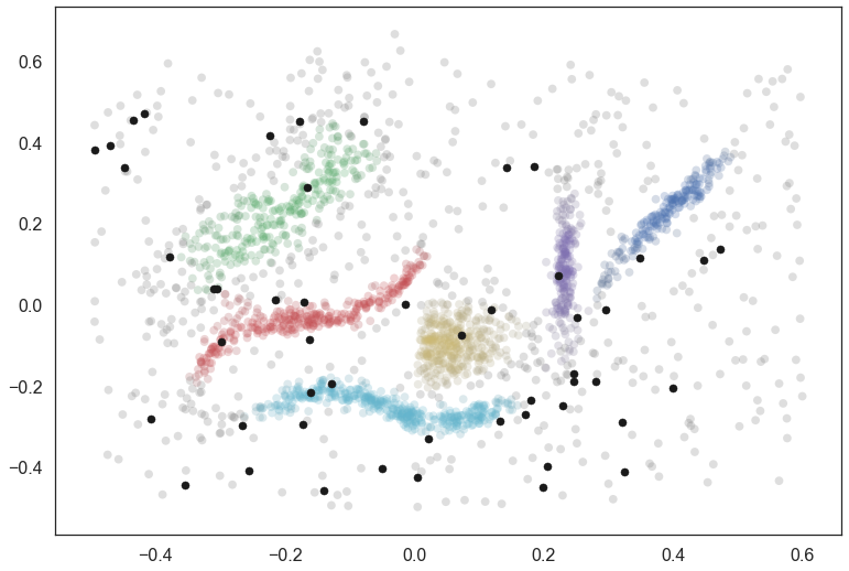
Now to make things a little more interesting let’s generate 50 new data points scattered across the data. We can plot them in black to see where they happen to fall.
test_points = np.random.random(size=(50, 2)) - 0.5

colors = [sns.desaturate(pal[col], sat) for col, sat in zip(clusterer.labels_,
                                                            clusterer.probabilities_)]
plt.scatter(data.T[0], data.T[1], c=colors, **plot_kwds);
plt.scatter(*test_points.T, c='k', s=50)
We can use the predict API on this data, calling
approximate_predict() with the HDBSCAN object,
and the numpy array of new points. Note that
approximate_predict() takes an array of new
points. If you have a single point be sure to wrap it in a list.
test_labels, strengths = hdbscan.approximate_predict(clusterer, test_points)
test_labels
array([ 2, -1, -1, -1, -1, -1,  1,  5, -1, -1,  5, -1, -1, -1, -1,  4, -1,
       -1, -1, -1, -1,  4, -1, -1, -1, -1,  2, -1, -1,  1, -1, -1, -1,  0,
       -1,  2, -1, -1,  3, -1, -1,  1, -1, -1, -1, -1, -1,  5,  3,  2])
The result is a set of labels as you can see. Many of the points as classified as noise, but several are also assigned to clusters. This is a very fast operation, even with large datasets, as long the HDBSCAN object has the prediction data generated beforehand.
We can also visualize how this worked, coloring the new data points by the cluster to which they were assigned. I have added black border around the points so they don’t get lost inside the clusters they fall into.
colors = [sns.desaturate(pal[col], sat) for col, sat in zip(clusterer.labels_,
                                                            clusterer.probabilities_)]
test_colors = [pal[col] if col >= 0 else (0.1, 0.1, 0.1) for col in test_labels]
plt.scatter(data.T[0], data.T[1], c=colors, **plot_kwds);
plt.scatter(*test_points.T, c=test_colors, s=80, linewidths=1, edgecolors='k')
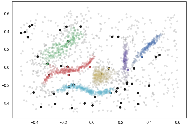
It is as simple as that. So now you can get started using HDBSCAN as a streaming clustering service – just be sure to cache your data and retrain your model periodically to avoid drift!