Soft Clustering for HDBSCAN*
Soft clustering is a new (and still somewhat experimental) feature of the hdbscan library. It takes advantage of the fact that the condensed tree is a kind of smoothed density function over data points, and the notion of exemplars for clusters. If you want to better understand how soft clustering works please refer to How Soft Clustering for HDBSCAN Works.
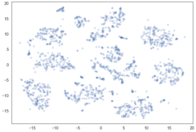
Let’s consider the digits dataset from sklearn. We can project the data into two dimensions to visualize it via t-SNE.
from sklearn import datasets
from sklearn.manifold import TSNE
import matplotlib.pyplot as plt
import seaborn as sns
import numpy as np
digits = datasets.load_digits()
data = digits.data
projection = TSNE().fit_transform(data)
plt.scatter(*projection.T, **plot_kwds)
Now we import hdbscan and then cluster in the full 64 dimensional space.
It is important to note that, if we wish to use the soft clustering we
should use the prediction_data=True option for HDBSCAN. This will
ensure we generate the extra data required that will allow soft
clustering to work.
import hdbscan
clusterer = hdbscan.HDBSCAN(min_cluster_size=10, prediction_data=True).fit(data)
color_palette = sns.color_palette('Paired', 12)
cluster_colors = [color_palette[x] if x >= 0
                  else (0.5, 0.5, 0.5)
                  for x in clusterer.labels_]
cluster_member_colors = [sns.desaturate(x, p) for x, p in
                         zip(cluster_colors, clusterer.probabilities_)]
plt.scatter(*projection.T, s=50, linewidth=0, c=cluster_member_colors, alpha=0.25)
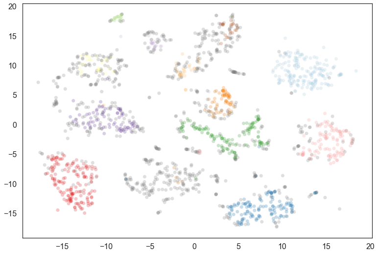
Certainly a number of clusters were found, but the data is fairly noisy in 64 dimensions, so there are a number of points that have been classified as noise. We can generate a soft clustering to get more information about some of these noise points.
To generate a soft clustering for all the points in the original dataset
we use the
all_points_membership_vectors() function
which takes a clusterer object. If we wanted to get soft cluster
membership values for a set of new unseen points we could use
membership_vector() instead.
The return value is a two-dimensional numpy array. Each point of the
input data is assigned a vector of probabilities of being in a cluster.
For a first pass we can visualize the data looking at what the most
likely cluster was, by coloring according to the argmax of the
probability vector (i.e. the cluster for which a given point has the
highest probability of being in).
soft_clusters = hdbscan.all_points_membership_vectors(clusterer)
color_palette = sns.color_palette('Paired', 12)
cluster_colors = [color_palette[np.argmax(x)]
                  for x in soft_clusters]
plt.scatter(*projection.T, s=50, linewidth=0, c=cluster_colors, alpha=0.25)
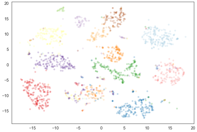
This fills out the clusters nicely – we see that there were many noise points that are most likely to belong to the clusters we would expect; we can also see where things have gotten confused in the middle, and there is a mix of cluster assignments.
We are still only using part of the information however; we can desaturate according to the actual probability value for the most likely cluster.
color_palette = sns.color_palette('Paired', 12)
cluster_colors = [sns.desaturate(color_palette[np.argmax(x)], np.max(x))
                  for x in soft_clusters]
plt.scatter(*projection.T, s=50, linewidth=0, c=cluster_colors, alpha=0.25)
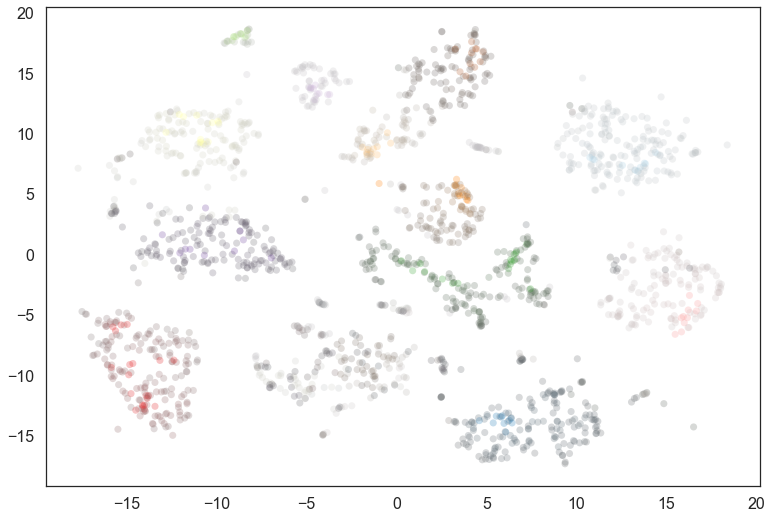
We see that many points actually have a low probability of being in the cluster – indeed the soft clustering applies within a cluster, so only the very cores of each cluster have high probabilities. In practice desaturating is a fairly string treatment; visually a lot will look gray. We could apply a function and put a lower limit on the desaturation that meets better with human visual perception, but that is left as an exercise for the reader.
Instead we’ll explore what else we can learn about the data from these cluster membership probabilities. An interesting question is which points have high likelihoods for two clusters (and low likelihoods for the other clusters).
def top_two_probs_diff(probs):
    sorted_probs = np.sort(probs)
    return sorted_probs[-1] - sorted_probs[-2]

# Compute the differences between the top two probabilities
diffs = np.array([top_two_probs_diff(x) for x in soft_clusters])
# Select out the indices that have a small difference, and a larger total probability
mixed_points = np.where((diffs < 0.001) & (np.sum(soft_clusters, axis=1) > 0.5))[0]
colors = [(0.75, 0.1, 0.1) if x in mixed_points
          else (0.5, 0.5, 0.5) for x in range(data.shape[0])]
plt.scatter(*projection.T, s=50, linewidth=0, c=colors, alpha=0.5)
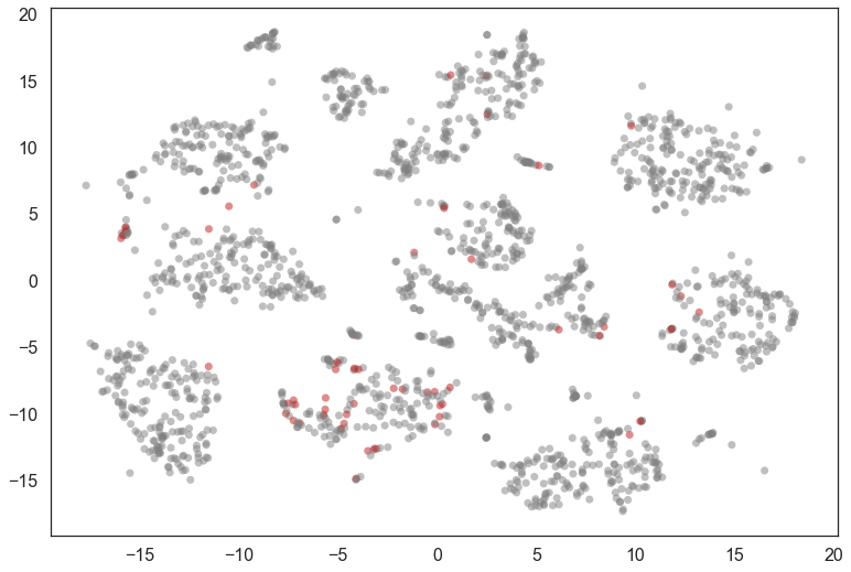
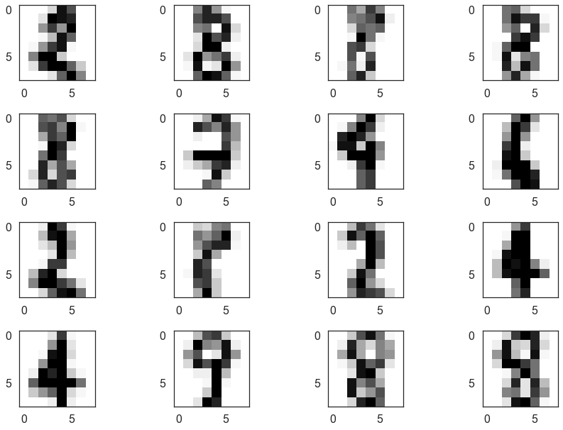
We can look at a few of these and see that many are, indeed, hard to classify (even for humans). It also seems that 8 was not assigned a cluster and is seen as a mixture of other clusters.
fig = plt.figure()
for i, image in enumerate(digits.images[mixed_points][:16]):
    ax = fig.add_subplot(4,4,i+1)
    ax.imshow(image)
plt.tight_layout()
There is, of course, a lot more analysis that can be done from here, but hopefully this provides sufficient introduction to what can be achieved with soft clustering.